Lookup on Each Duplicate Value in Excel
One of the shortcomings of Excel’s lookup functions is that you can’t match on duplicate values, instead the functions only match on the first instance of the lookup value it finds in a column or row. This tutorial will provide you with a solution to this shortcoming. The formula is fairly involved but I will break it down into steps to make it easier to understand. Download the example file here.
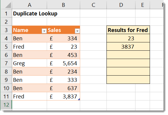
In our example we have a sales table and a second table listing sales for a specific salesperson. When we change that name at the top of the second table the formula will return the sales values for that person. The formula returns 5 results for Ben, for Fred it would return 2 and Greg, 1.

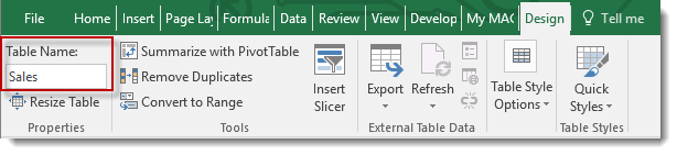
The first table has been converted into an Excel Table. You can do this fairly simply by clicking anywhere in it and then using the shortcut key CTRL T. The table has been named Sales. To name a table, click on the DESIGN tab on Ribbon: the Table Name option is on the far left of the Ribbon as shown below.
The steps involved in putting this formula together may not seem to make sense initially but stick with it and you will see how everything fits together. The formula is being written in cell D4.
STEP 1 – Return Each Row Number in our Sales Table
The first step is to return each row number within the sales table. We can use the ROW function to achieve this. =ROW(Sales[Name])-3
Normally ROW returns the row number for a single cell: we have specified the entire Name column. The -3 has been included at the end of the formula as the table starts in row 4 of the worksheet. The result of the formula is 1. However, as we have asked the ROW function to return the row number of all the cells in the Name column we have to use the F9 trick to see the true result.
The F9 trick requires you to select the text of the formula and then press the F9 function key on your keyboard. You should then see this:
={1;2;3;4;5;6;7;8}
The formula is in fact returning each row number. At the moment the row numbers are hard-coded into your formula as a result of using the F9 trick. You will need to undo this (CTRL Z) to get back to the original formula.
STEP 2 – Only Return the Row Numbers for the Sales Person Specified
The second step is to get Excel to only return row numbers where the specified sales person’s name appears. The name Ben is in cell E3 in our example.
=IF(Sales[Name]=E$3,ROW(Sales[Name])-3)
The result is again 1 but using our F9 trick we can see what the formula is actually returning:
={1;FALSE;3;FALSE;5;6;7;FALSE}
So the IF function is only performing the ROW calciulation where the logical test is met – as in the name is equal to Ben.
STEP 3 – Return Each Row Number As the Formula is Copied Down
Now we know which rows Ben appears in we need each row number to be returned independently as we copy the formula down the second table.
We can use the SMALL function to achieve this. SMALL returns the k-th smallest value in a data set. The data set or array is returned by our current formula, the k-th smallest value can be specified with a simple incrementer – ROWS(D4:D$4) which when copied down will return 1, 2, 3 etc.
So the formula at this stage will look like this:
=SMALL(IF(Sales[Name]=E$3,ROW(Sales[Name])-3),ROWS(D4:D$4))
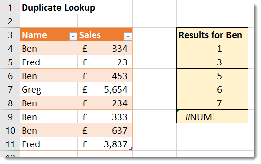
If you copy the formula down the table you will see it returns the correct row numbers for Ben.
NB: The formula only works as an array formula so you need to use CTRL SHIFT ENTER to confirm the formula and then copy it down. As an array formula brace brackets will appear around it.
STEP 4 – Return the Sales Values for the Specified Sales Person
We need the INDEX function to return values from the Sales Column in the same vertical position as each occurrence of Ben’s name in the Name column.
=INDEX(Sales[Sales],SMALL(IF(Sales[Name]=E$3,ROW(Sales[Name])-3),ROWS(D4:D$4)))
Copying the formula down as an array formula your table should now look like this.
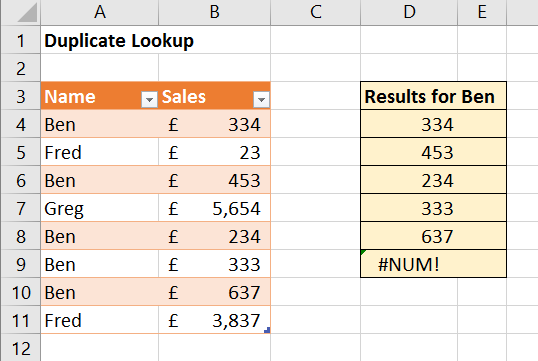
STEP 5 – Return the Correct Number of Sales Values
The final step is to avoid the #NUM! error which occurs when too many sales results are returned for the specified salesperson. The IF function’s logical test compares an incremented value (a count of the number rows the formula has been copied to) with a count of the number of times Ben’s name appears in the Name column. If the count of the number of rows exceeds the number of times Ben’s name appears the IF returns an empty text string.
=IF(ROWS(D$4:D4)<=COUNTIF(Sales[Name],E$3),INDEX(B$4:B$11,SMALL(IF(A$4:A$11=E$3,ROW(Sales[Name])-3),ROWS(D$4:D4))),””)
The formula needs to be entered as an array formula before it can be copied down.
Try changing the name entered in E3 and the relevant sales values will appear as below.