If you need to analyse a list or database in Excel you should convert your data into an Excel Table. This tutorial will show you how to convert your data into an Excel Table and then look at the advantages of doing so.
Data that is suitable for conversion into an Excel table, looks pretty much like this.
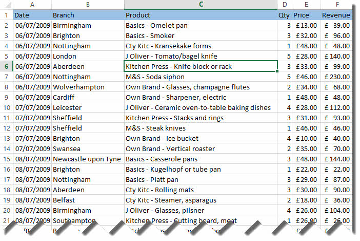
Each column has a column header and each row represents one record in the database. You are best off deleting any blank rows or columns within your data.
You can download this sample file if you want follow the tutorial.
Converting a Range into an Excel Table
To convert your data into an Excel Table, first click into any cell in your data and then click on the INSERT tab on the Ribbon and click the Table button.

CTRL T is the shortcut for creating an Excel Table.
Excel will ask you to confirm where your data is and also that it contains headers.
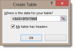
Click OK to confirm.
So what do you get with an Excel Table?
1. Drop-Down Filters
Just like when you apply a filter to a list, an Excel Table shows drop-down lists in the column headers which allow you to filter your data.

2. Column Headings are Always Visible
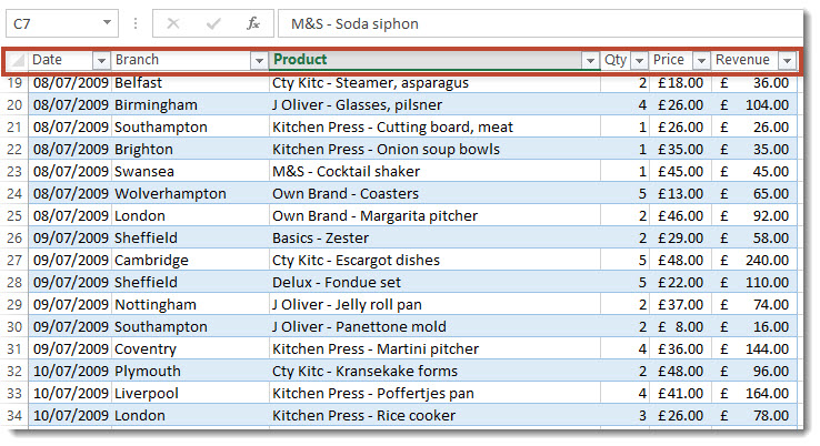
When you scroll down your data and the row with your column headers disappears off the screen, the column headings and filter drop-downs appear in the column titles (A, B, C, D etc). By the way if this isn’t working for you – make sure you have clicked into your data before you try.
3. Automatic Totals – Even When You Filter!
When you create an Excel Table, you get an extra tab on your Ribbon called DESIGN. On the DESIGN tab is a really useful option called Total Row. Tick this option to have your Excel Table perform calculations on fields in your data.

As you will see in the image below, the last row of my Excel Table now includes a total for revenue: that calculation was added automatically. I can add a calculation to each column in the Total Row by selecting a function from the drop down list which appears in the cell when I select it (see below).

When you apply a filter to your table, these totals will adjust to calculate only on the visible records.
4. Banded Rows – to Make Your Data Easier to Read
You will have noticed that every other row in my table is shaded. Makes the data easier to read, doesn’t it? This shading is automatically applied. You can change the formatting applied to Excel Tables on the DESIGN tab.

Notice you can also have banded columns. If you would prefer a different colour scheme, choose another Table Style from the gallery.
5. Dynamic Named Range Created Whenever you Create a Table
This is one of the biggest benefits of creating an Excel Table. Firstly, notice the Table Name property on the far left of the DESIGN tab – see below. Your table has a name! By default the table is called Table1 – not exactly imaginative. You can rename your table to whatever you like, but avoid spaces and make the first character a letter.

So what? You can name your table. Well it is quite useful to have a name that refers to all the data in your Excel Table, especially when you need to define a range for a chart or PivotTable. With my table named there is a more convenient way of referring to it than using =$A$1:$F$17860.
One of the major benefits of using an Excel table is that it will automatically expand when you add a new record – even if it is added at the end of the table. So the range of cells that your name refers to will also automatically expand. This is known as a dynamic range.
To add a new record to an Excel Table, click into the last cell of the last record (above your Total Row if you are displaying it) and then press the TAB key on your keyboard.

Using the TAB key creates a blank row. The blank row is still within the table – pretty obvious in my example (above) as it’s above the Total Row, but notice in the bottom right-hand corner – a small blue handle and thin blue border – this is the boundary of your table. This boundary always expands when you add new records.

This also works when you add new columns. In the image below, you can see I have added an additional column called Discounts. The table has automatically expanded to include the new column including applying the shading.

6. Magic Formulas
Not quite magic, but nearly. When you add a formula to a column in an Excel Table, look what happens…
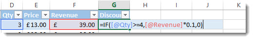
Instead of displaying a cell address for the Qty cell, when I selected the cell for my formula, the Excel Table entered [@Qty]. The same format for referring to a cell was applied to the Revenue reference [@Revenue]. Makes the formulae easier to read, I think.
What is really clever is that when I confirm the formula it automatically gets copied into the rest of the column without me having to do a thing.
Magic Formulas Outside Your Table
Here are some differences in formulas that you create outside an Excel table but which refer to ranges inside an Excel Table.
In the example below I have started to create a SUMIFS formulae to add up all the revenue for a particular branch. I want to refer to the column names rather than try and select the 17,000 rows in each column. I’ve typed the “t” and the AutoComplete list shows me the table name Table1. I can double-click to complete the name.

I then enter an opening square bracket and the AutoComplete list shows the field names in my Excel Table.

Again I can double-click to complete but I need to close the square bracket manually.
I can continue to refer to columns within the table as shown below. Note always precede the column name with the Table Name.

7. Create a Dynamic Range for Charts & PivotTables
We now know that Excel Tables create a dynamic range. Well if you create a chart based on an Excel Table, you can add new records and the chart will automatically update to show the new data.
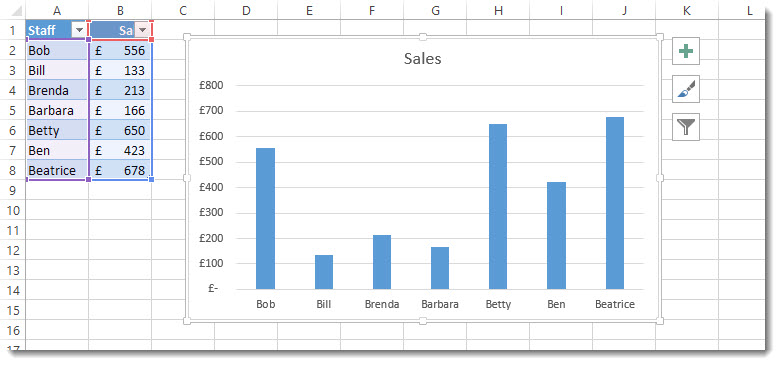
Here’s my chart with the original data. The data is in an Excel Table.
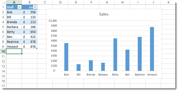
I add Howard’s sales figures and the chart automatically updates without me having to redefine the data range.
The same is true for PivotTables – if you base the PivotTable on an Excel Table it will pick up new records you enter in the underlying data when you refresh the Pivot cache. See our video on creating a dynamic range for a PivotTable.