The GETPIVOTDATA function is really useful if you want more control over the format and layout of the data that your PivotTable generates.
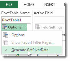
You need to make sure that Excel is setup to use the function. With your PivotTable selected, on the ANALYZE Ribbon tab, open the Options menu and make sure Generate GetPivotData is ticked.
Whenever you reference a cell within the “values” / “data” area of a PivotTable, outside of the PivotTable, Excel generates a GETPIVOTDATA formula – see below.
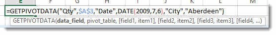
The Function use the following arguments:
- data-field – the name of field whose data you want to retrieve
- pivot_table – a reference to cell within the PivotTable you want to retrieve data from. By default Excel uses the top left cell as a reference
- field, item – pairs of fields and item names that describe what data you want to retrieve
Watch the video to see how you can swap these hard coded field and item pairs with cell references to column and row headings within your own tables.