The most likely occurrence of the #N/A error is when you are using one of the lookup functions such as VLOOKUP or MATCH. The error is telling you that what you are looking up cannot be found. So the error is not an error in the conventional sense as it is telling you something useful. Below are some notes on dealing with the #N/A error, but take a look at our video below which shows some useful examples.
If you were using VLOOKUP to compare two lists to find out which items appeared in both, then you know you can discount the items that return a #N/A error. You can then filter these out or delete them depending on your scenario.
A VLOOKUP function has two modes or ways of working. It can either perform an exact match or an approximate match. The #N/A error will appear for different reasons depending on the mode you are using.
With an exact match, you need to state FALSE in the fourth and final argument.
eg =VLOOKUP(A1,B1:C10,2,FALSE)
You would use an exact match (as the name suggests) to exactly match values across two tables. If the match is not found the #N/A error is returned.
Sometimes two values appear to the eye to match but the VLOOKUP says they don’t. This could be because of trailing spaces in one of the values. Use the TRIM function to remove leading and trailing spaces from a text string. TRIM will also remove superfluous spaces between characters where there is more than one consecutive space. If your lookup value contains the offending space or spaces then trim it within the VLOOKUP, such as =VLOOKUP(TRIM(A1),B1:C10,2,FALSE). If the spaces are in the lookup table you might need to TRIM the values in a separate column and then replace the originals with these using paste values.
However if there is no match then #N/A is, as mentioned above, useful. The error does however make you worksheet look wrong. If this bothers you, use the IFERROR function to replace the error with a value. So for example =IFERROR(VLOOKUP(A1,B1:C10,2,FALSE),“NOT FOUND”) returns NOT FOUND if the VLOOKUP cannot match a value or returns the result of the VLOOKUP if it can.
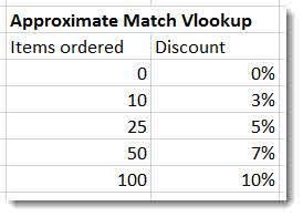
An approximate match works slightly differently: in the first column of your lookup table you would enter values to express ranges. In the example below the first column arranges the numbers in ascending order so that 0 – 9 would return a discount of 0% and 10- 24 would return a discount of 3% etc. So if I looked up a value of 11 using an approximate match instead of returning the #N/A error (as it would with an exact match) it would return 3%.
An approximate match does not need to use the fourth and final argument so it might look like this: =VLOOKUP(A1,B1:C10,2)
The #N/A error can occur when using an approximate match but for different reasons. It will occur if the value you lookup is less than the lowest value in the first column of the lookup table and it might occur if the first column is not arranged in ascending order – you should always arrange the first column in ascending order for an approximate match!