In previous versions of Excel there have been a number of different ways of filtering on dates within a PivotTable. In Excel 2013, Microsoft have gone and added another: Timelines.
Timelines provide a more graphical way of filtering your PivotTable when filtering based on a date field in your underlying data. You can choose whether your Timeline shows years, quarters or months or days – depending on the level of detail you wish to filter on. Although Timelines provides a nice graphical interface that is more intuitive to use than a normal date filter – they have their limitations as I discuss below. Please also note that the Timeline feature will not work on a normal range or Excel Table.
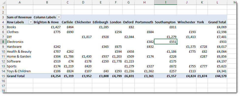
In the example below, my PivotTable includes row and column headings for products and branch location respectively. The values show a sum of sales for each branch.
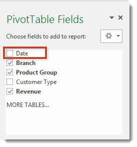
In my field list, you will see there is a date field – this is necessary if you are going to use a Timeline (kind of makes sense!)
Creating your Timeline
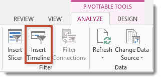
To create a Timeline, first click somewhere in your PivotTable and then select the ANALYZE tab on the Ribbon. The Insert Timeline button is found in the Filter group.
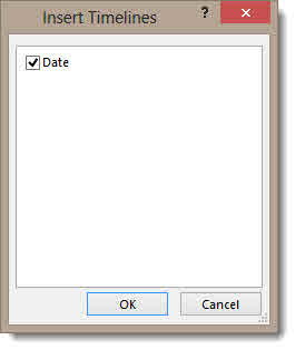
Once you have clicked the button, Excel then asks you to select the date field that you want your Timeline to filter. Click on OK once you have checked the relevant field. I’ve only got one date field, but I still have to make the selection.
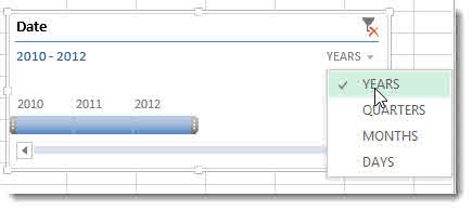
Your Timeline can be configured to group dates by years, quarters, months or days. Use the drop-down list, top right of the timeline to select your required grouping as shown below. In my example I have grouped the dates by years.
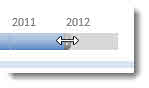
To apply a filter via the Timeline, adjust the blue bar by dragging the end handles as shown below.
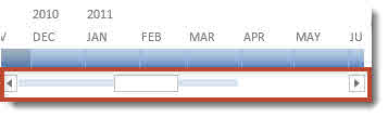
If I group by months, I am forced to use the scroll bar at the bottom of the timeline to view all the months. Not a major problem, but just be aware that the scroll bar is there for when you have a lot of dates.
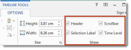
You can control the visibility of the scroll bar and other elements in the Timeline window up on the OPTIONS tab on the Ribbon. If the OPTIONS tab is not visible then you need to activate it by selecting your Timeline.
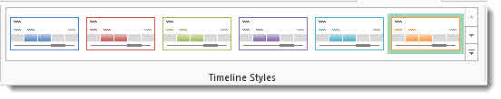
If you are not happy with your Timeline’s colour theme, then you can easily change it using Timeline styles, also up on the OPTIONS tab.
Timelines vs Slicers
For those of you who have used Slicers before you may be wondering if the Timeline replaces Slicers for date fields. Well not quite: although using Slicers to filter on years, quarters and months takes a little bit more set up, they are more flexible as you can select non-contiguous items.
Apart from taking more time to setup, Slicers also take up more space on your spreadsheet, so I guess Timelines do have their advantages.
In order to create Slicers for each grouping of the dates, you will need to first of all group the dates in the PivotTable itself. Once the grouping has been established, a field is created for month, quarter & month (or whichever groups you created). Slicers can then be created based on these fields. If you are not sure how this is achieved, watch the video above.