Slicers create a visual dashboard that enable you to analyse and filter your data. Slicers were first introduced in Excel 2010 but were only made available for PivotTables. Excel 2013 makes Slicers available for the filtering of regular Excel tables. Download the featured file here.
Converting Your Range into an Excel Table
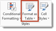
First things first, you can only connect slicers to an Excel table opposed to a range. A range is just a bunch of regular contiguous cells that you happened to enter some data in. To convert a range to an Excel table: click in any cell in your range and then on your HOME tab in the Styles group, click the Format as Table option.
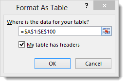
You then get a choice of styles for your Excel table (I bet you feel spoilt rotten). Select which style you want to use and then click OK in resulting dialog to confirm the range you want to convert.
Your table will now include filter buttons on each column heading plus the formatting you chose with your preferred style.
Connect your Excel Table to some Slicers
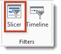
The next thing to do is to connect your Excel table to some Slicers. Click into any cell in your Excel table and then on the INSERT tab in the Filters group click the Slicer option.
In the Insert Slicers dialog, select which Slicers you want to create: this would be for whichever fields you might want to filter on. Click on OK to confirm.

Formatting Slicers
Your Slicers will now need to be repositioned and resized on your worksheet. You can also change the colour and number of columns within the Slicer.
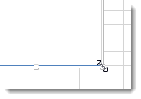
To move a Slicer drag it either from its title bar or from an empty space below the values. To resize a Slicer, drag one of the resizing handles around its border
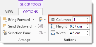
To change the number of columns displayed in a Slicer, click on the OPTIONS tab and in the Buttons group change the value for the number of columns.
To change the colour of your Slicer, select one of the Slicer styles. These again appear in the OPTIONS tab.

Here’s an example of a Slicer with three columns and with the red Slicer style applied to it.

Filtering Your Table Using Slicers
To filter your table using Slicers just click on the relevant buttons within the Slicers to filter on that value. You can select more than one value to filter on by holding the SHIFT key to select contiguous items or hold down CTRL to select non-contiguous items. You can also create a filter selecting buttons from more than one Slicer (you don’t need to use SHIFT or CTRL to do this).
To clear a filter click the Clear Filter button that appears top right of a Slicer.

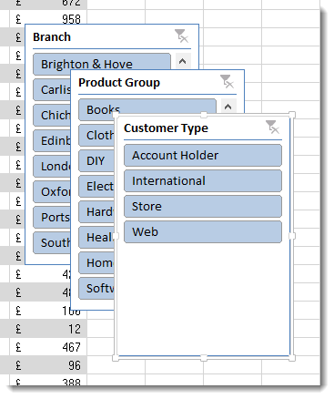
One nice feature of using multiple slicers is that they report to each other. In the screen dump below you will see that the Branch Slicer is filtering my Excel table for London sales. The Customer Slicer automatically reports that there were no Web sales and the Product Slicer reports no sales for Books, DIY, Electronic and Sports.
