This tutorial will show you how to format cells using custom number formats that include icons and emojis. Conditional formatting as you may know provides a limited selection of icon sets, but if you are after more variety or indeed a bit of fun with your Excel spreadsheet then this is for you. Download the featured file here – Custom Number Formats
A video tutorial is also available at the bottom of this page.
Example 1
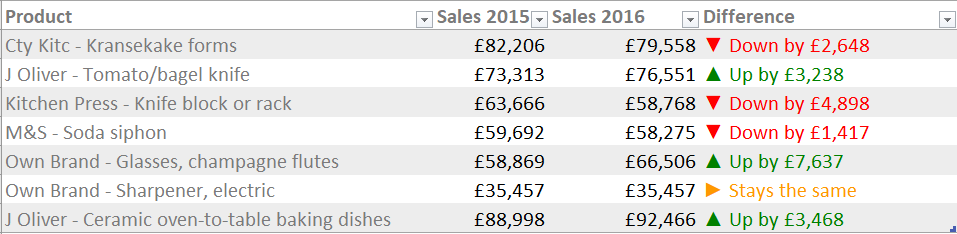
In our first example we want to indicate whether sales figures have increased or decreased. We are going to use a mixture of icons and text to achieve this.
You can take a peak at existing custom formats by opening the Format Cells dialog, with the shortcut CRTL 1.
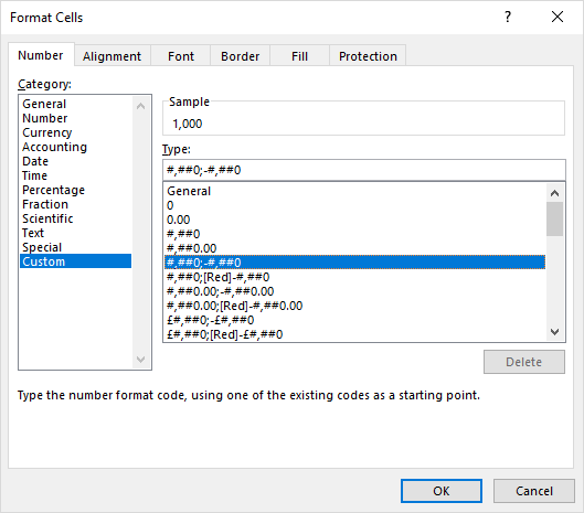
There are for four formats that can be applied to a cell: one for positive values, one for negative values, one for zero values and then one for text values.
Not all formats use all four parts as you can see. The order, however, is always the same. Notice how the different parts are separated with a semi-colon.
“Positive Values” ; “Negative Values” ; “Zero Values” ; “Text Values”
If you only use the first two parts of the format – the positive and negative value parts, the zero values assume the same format as the positive value.
In our example we want positive values to be displayed with an ‘up’ triangle followed by the text “Up by”, followed by the calculated difference between the two years – the formula in the cell. So we would use this code: [Color10] “▲ Up by ” £#,### (explanation below).
Explanation of [Color10] “▲ Up by ” £#,###
[Color10] refers to the colour you want to display the font in. There are 56 colours you can specify – see the table below.

“▲ Up by “ is the text (including icon) that you want to display alongside the cell’s value – this must be enclosed in speech-marks. The icons needs to be pasted into the format code – but first you need to create them.
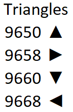
Create icons in your worksheet using the UNICHAR function. For example to return the ‘up’ triangle use the following formula =UNICHAR(9650), then convert the formula to a value (copy | paste values) before then copying it into your custom format code.
Here are the rest of the UNICHAR numbers.
£#,### – the last bit of our code tells Excel how to display the result of the cell’s formula. Here we want a currency symbol and a thousand separator.
The full code for our custom format is as follows. Don’t forget the order of the formats – positive values; negative values; zero values.
[Color10] “▲ Up by ” £#,###;[Color3] “▼ Down by ” £#,###;[Color45] “► Stays the same”
Here it is in the format cells dialog.

Example 2
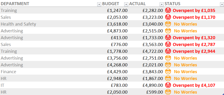
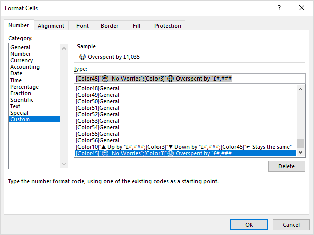
In our second example we need to indicate whether an account is over budget: emojis have been used within the custom format.
You can create the emoji characters with the UNICHAR function just as you did the triangles. Here are UNICHAR numbers you will need.

The code for this custom format is [Color45] “???? No Worries” ;[Color3] “???? Overspent by ” £#,###
That’s it – have lots of fun with your icons and emojis!
Here are some more UNICHAR numbers for you.

Watch our video tutorial on this topic.