Replace Text in Excel using SUBSTITUTE & REPLACE

Replacing Text using the SUBSTITUTE and REPLACE Functions

Watch the video and/or follow the tutorial below. There are two functions in Excel that allow you to replace text in a text string.

SUBSTITUTE allows you to specify the content you want to replace – for example you may want to replace all hyphens in a product code with a space.

REPLACE allows you specify the position within a text string where you want to replace and also allows you to specify the number of characters. So you could replace first name last name with first name initial last name.

SUBSTITUTE & VLOOKUP

You could use SUBSTITUTE in conjunction with a VLOOKUP. For example, I have a master list of product codes and associated prices.  I have a separate table of product orders that I want to automatically price using a VLOOKUP.  At the moment the VLOOKUP will not work because the product codes in the order list (column D) contain hyphens.

To remove all the hyphens I would use the following formula:

=SUBSTITUTE(D2,”-“,” “)

The first argument (Text) asks you specify the text string that you want to perform the replacement within, in my example that’s D2.

The second argument (Old_text) asks you to specify the character or characters you want to replace, in our example that’s the hyphen.  Note, the double-quotes around the hyphen “-“

The third argument (New_text) asks you to specify the character or characters you want to use to replace the old_text. In our example that’s a space – note again the double hypens. “ “

The fourth argument (Instance_number) allows you specify which occurrence of the old_text you want to replace.  If left empty, as with this example, it will replace all occurrences, but for if I entered 2, it would only replace the second hyphen.

To return the correct price for each product I would nest the SUBSTITUTE function within my VLOOKUP, like this.

=VLOOKUP(SUBSTITUTE(D2,”-“,” “),$A$1:$B$200,2,FALSE)

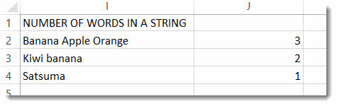
Count the Number of Words in a Text String Using SUBSTITUTE

You can use the SUBSTITUTE function in conjunction with the LEN function to count the number of words in a text string.  This might be helpful if you want to count the number of products that have been ordered (where the products have been entered into a single cell).

To calculate the number of words we need to calculate the number of spaces in the text string.  The calculation works like this: calculate the number of characters in the text string including spaces then calculate the number of characters excluding spaces, then subtract one from the other.

The LEN function returns the number of spaces in a text string, so LEN(I2) would calculate the number of characters in I2.

To calculate the number of characters excluding the spaces we would use LEN and SUBSTITUTE: LEN(SUBSTITUTE(I2,” “,””)) where the SUBSTITUTE function replaces spaces with an empty text string (two double quotes with nothing between).

So the subtraction looks like this: =LEN(I2)-LEN(SUBSTITUTE(I2,” “,””))

Now, if there are three words, there are two spaces, if there are five words there are four spaces and so on.  So the calculation needs a little tweak: with a +1 at the end: =LEN(I2)-LEN(SUBSTITUTE(I2,” “,””))+1, we have the right answer.

REPLACE Function

The REPLACE function has four arguments:

Old_text – the text that contains the characters you want to replace

Start_number – the position of the first character in the Old_text that you want to replace

Num_chars – the number of characters you want to replace.  If 0, no characters are replaced

New_text – the replacement text

In this example we are going to use REPLACE to convert first name last name to last name. I appreciate that there are numerous ways this can be done in Excel, but let’s have a go with REPLACE.

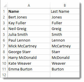
The formula used to achieve this is =REPLACE(A2,1,SEARCH(” “,A2),””)

Old_text = A2

Start_number = 1

Num_chars – this is more difficult as we want to replace the whole of the first name and the first names in our list have different character lengths.  The solution is to use the SEARCH function to find the position of the space which gives us the number of characters to replace. SEARCH(” “,A2)

New_text – we want to delete the first name so need to it with an empty character string “”

Example 2

We could also use REPLACE to convert first name last name to first name initial last name as shown below.

The formula for this would be =REPLACE(A2,1,SEARCH(” “,A2)-1,LEFT(A2,1)

As with the previous example Num_chars uses the SEARCH function to search for the space, but then substracts one, so that the space preceding the last name is not replaced.  The New_text argument uses the LEFT function to return the initial in the first name.

Please note that you can opt to enter zero in the Num_chars argument.  This would mean your New_text would not replace existing characters but would just be added at the specified position.

So for example =REPLACE(A2,1,0, “Mr “) would return Mr Bert Jones Effectively you are not replacing anything you are actually concatenating or joining values.