Introducing the Data Model

One of the new features included in Excel 2013 is the Data Model. The Data Model is a cut down version of the PowerPivot add-in that was and is still available for Excel 2010 users. The PowerPivot add-in allows you to combine multiple tables in a PivotTable.

In Office 2013 the PowerPivot add-in is only available to Office 2013 Professional Plus users – not a licence you can buy retail. However, the Data Model (the cut down version of the add-in), is available to standard Excel 2013 users: this tutorial explains how to use the Data Model to combine multiple, related tables in a Pivot Table.

In many ways the Data Model achieves the same thing as a VLOOKUP: it combines data from multiple sources based on a common field. The Data Model is probably the way to go if you are working with a lot of records and a lot of fields where working with a VLOOKUP would be more time consuming and awkward. Anyway, let’s have a look at how to use the Data Model.

The video below will take you through this exercise and you can download the featured file to practice your new found knowledge!

The solution I want to reach using the Data Model concerns these three sets of data. The first contains records of sales transactions

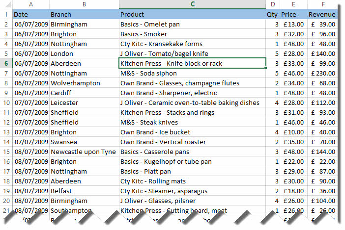
The second set of data assigns a product category to each product

The third set of data tells me which region each branch is in.

I need my PivotTable to show me a breakdown of sales per product category, per region – something I can’t do with the original sales data because the both the product category and region information are missing.

Converting Ranges to Excel Tables

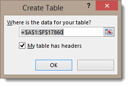
[dropcap type=”circle” color=”#ffffff” background=”#66a3bf”]T[/dropcap]he three sets of data are in the same workbook on different sheets. To start with I am going to convert each range into an Excel table: this makes the data easier to identify in the Data Model as I can name the tables.

To convert a range is pretty easy. I just select a cell within the data and then on the INSERT tab on the Ribbon click the Table button.

I then need to click OK to confirm I am happy with range selected.

Your Excel table will include some formatting and the filter drop-downs for each column: we won’t need the filter functionality but it’s applied anyway. The important thing to do at this stage is to name the table. You will notice that your Ribbon now includes a Table Tools DESIGN tab. On the far left of the Ribbon with that tab activated you will see a box where you can enter a name for the table. By default it will be called Table1. I named my first table Sales_Data. Spaces are not allowed in table names so I used an underscore.

You need to convert each of your ranges to a table, naming them accordingly. I named my other two tables Product_Data and Region_Data.

Adding the Tables to the Data Model

[dropcap type=”circle” color=”#ffffff” background=”#66a3bf”]T[/dropcap]he next step is to add my tables to the Data Model. If I add one of them, they all get added at the same time.

I am going to start off by adding the sales data to the Data Model. To do this, I click into any cell in the data and then on the INSERT tab on the Ribbon click the Pivot Table button.

The important thing here is to check the option that allows you to add the data to the Data Model (see below).

Click OK to confirm.

A PivotTable appears on a new worksheet and in the PivotTable Fields list you will notice two buttons: ACTIVE and ALL. Click on the ALL button and you will see that each table has been added to the Data Model.

Establishing Relationships between the Tables

[dropcap type=”circle” color=”#ffffff” background=”#66a3bf”]A[/dropcap]lthough the fields have been added to the Data Model I still need to establish relationships between the data.

The sales data is related to the product data via the product field (the product names appears in each table). The sales data is related to the region data via the branch field (again, the branch names appear in both tables). By establishing a relationships between the two tables I will be able to connect branch with its respective region and product with its respective product category.

The relationships are set up on ANALYZE tab within the PivotTable Tools. Click the Relationships button within the Calculations group as shown below.

In the Manage Relationships dialog, click New and then pick the tables and fields you want to use to establish a relationship. In the example below I have established a relationship between the Sales_Data table and the Region_Data table using the common Branch field.

You have to get the direction of the relationship right. Notice the first field you select is called the Foreign column and the second the Primary Column. In each case with our example the Sales data contains the Foreign key and the other table (region or product) contains the Primary column – the data we are adding to our Sales data.

If you get the direction wrong Excel will let you know and it’s just a matter of swapping the columns around.

Click on OK to confirm the relationship. I now need to create a relationship between the Sales table and the Product table as shown below.

With the relationships established I can now close the Manage Relationships dialog and get on with adding fields to my PivotTable.

Creating the PivotTable

[dropcap type=”circle” color=”#ffffff” background=”#66a3bf”]I[/dropcap] need to expand the table buttons in the field list to see my table fields.

I can now add the fields to the PivotTable as I would normally. How to add and format fields is another tutorial altogether so I will assume you are already up to that.

To reach my original goal: get a breakdown of sales per region per product category, I arranged my PivotTable as shown below.

My PivotTable now provides the solution.

The Downside

There are a few downsides of using the Data Model:

you can’t group fields. Grouping fields is pretty essential if you are working with date fields
you can’t create calculated fields or items
you can’t double-click a value in a PivotTable get and see the records that make up that value on a separate sheet

Tina McGrath

Chester was a great trainer, I personally learnt so much in one day and it was all down to his calm, friendly demeanour and huge knowledge - we covered many areas which will help us to develop ourselves and the work we do. Thank you Chester, was lovely to meet you :-)

emmie BL

Myself and my team had an absolutely fab day with Chester going over excel - it was quite revelatory, with lots of really helpful hints & tips, great clear explanations and plenty of time to ask questions. Being able to work on things in real time, use our own data spreadsheets and his practice ones and have things properly explained has been so useful. Chester's a great instructor/facilitator - pitches to your needs and is very flexible. I would completely recommend him if you're needing to get a grip on all things excel! Thanks very much, Chester!

Martyn Lee

Chester was a great tutor understanding our needs and allowing time to understand and digest. Great humor too which always lightens a training day. Look forward to another session soon.

Angus Brown

Detailed, informative and fun, Chester made the class enjoyable and engaging - i have learnt a huge amount from the time we had together

Sisii de Winter

We booked Chester for several in-house training sessions including Fundamentals, Intermediate and Advanced Excel. He was brilliant with each, very inclusive and patient with all team members. Would fully recommend.

Lucy Maxwell Scott

A great online one on one intermediate training session in excel - the tools and activities Chester has developed and used are great. His teaching style was highly responsive to my needs (applications I wanted, my learning style). I would strongly recommend him - whatever your level of excel expertise and whatever level you are aiming for!

Louise Walpole

The online Excel Intermediate course I attended was really high quality. It was pitched at the right level with opportunity to work through examples as part of the course. Course material and follow up support has been excellent. I would highly recommend.

Savannah Baldry

Excellent training with Chester who's both knowledgeable and a great teacher. He takes the time to make sure you've understood before moving on and I was lucky enough to get some bespoke training specific to my needs. Thanks very much

ECA Account

I had an intermediate/bespoke excel course with Chester back last year, and enjoyed it so much and thought so highly of the course, I subsequently arranged beginners, fundamentals, intermediate excel courses and Microsoft PP/word courses for my colleagues. Even in a virtual setting Chester is clear in his delivery and guidance, exceptionally knowledgeable, and very adaptable to ever changing attendee lists or capabilities and requirements within the team. It will be great to put our new skills to good use. My advise to people, would be to take notes! Thanks Chester! Kathryn P.

Roofing Contractors Cambridge Ltd

An employee recently completed an online days training with Chester. He thoroughly enjoyed it and had a great learning experience. Fully recommend Blue Pecan Computer Training and would definitely use them again for future training.

Excel 2013 Combining Multiple Tables in a PivotTable using the Data Model